Statistical Analysis of Data on Traffic Accidents
I. Introduction
Abstract:
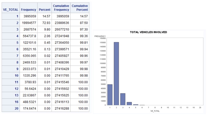
Traffic accidents inevitably affect our daily lives and we try our best to avoid those happen to our loved ones. As traffic data continues to grow, big data will likely play a large role in saving lives as it is instituted in cities and vehicles all around the world. In this report, we used General Estimates System (GES) data, which is a representative sample of police-reported motor vehicle crashes of all types collected by the National Highway Transportation Safety Administration (NHTSA) from years 1988 to 2013, as our main data source to perform statistical analysis.
In this study, we aim to identify variables that contribute to the injury severity level of victims when car accidents happen. Predictive models for injury severity level are developed. We also exploit outside data source such as living expense index to determine the average economic cost of accidents. Our ultimate goal is to develop a paradigm to envision the maximum injury severity level and potential economic cost under different circumstances if an accident happens.
II. Methodology
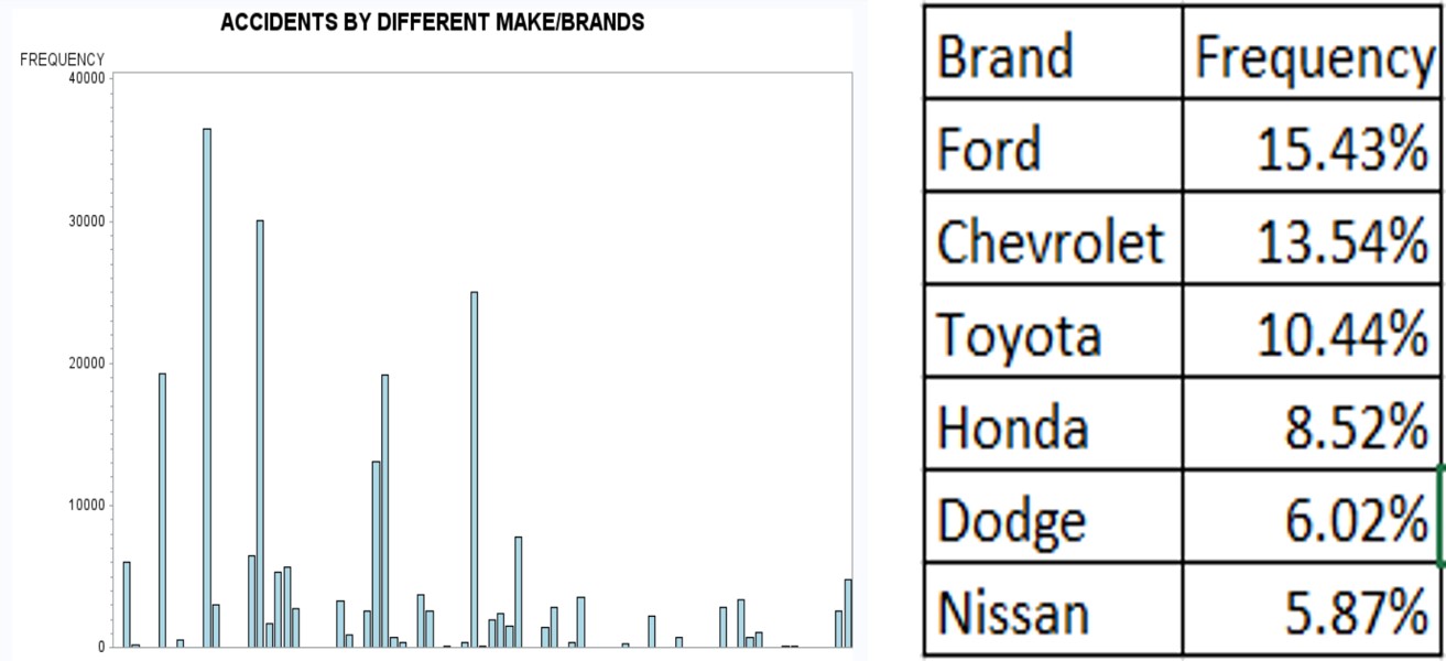
After deep investigation of the datasets, we are able to identity significant variables contributing to the injury severity level of someone in the car when accident happens. As we can tell from the flow diagram below, make, model of the vehicle, driving speed , gender, type of crash all relate to accident caused injury. We’ve also adopted outside data source to help us determine the average cost of certain injury type accident by state and leads us to conclusion of estimated economic cost of a certain vehicle accident.
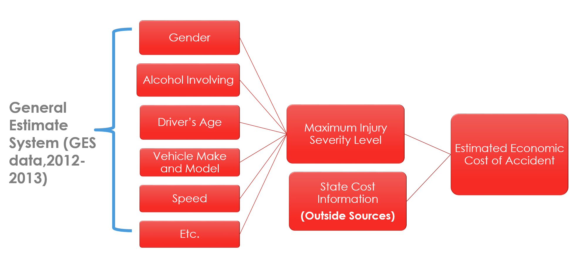
We also want to know the relationship between the economic cost of a car crash and the location where the accident happened along with the injury level of the driver. Here the definition of economic cost that we are using includes the medical cost of any necessary treatment and the damage repair fee on the vehicle. Since we already have the estimated injury level of the driver in a car accident, we used a imported outsource datasets to map our estimated economic cost of vehicle accident.
Our ultimate goal is to build an accident price explorer (APE) based on the GES datasets, in conjunction with other relevant outside resources. In practice, APE would allow readers to input conditions that are significant in contributing to a traffic accident assist readers to envision the maximum injury level that may possibly occur to someone in the vehicle under different accident circumstances and demonstrate the regional potential estimated economic cost of these crashes. We hope through our model and analytics, everyone would have a better understanding in what’s causing an accident and how much it would harm someone both physically and financially. We also believe APE could serve as a useful option for car buyers to check before making purchase options and provide a wider prospective for those who wanted to improve safety on the roads.
III. Data Management
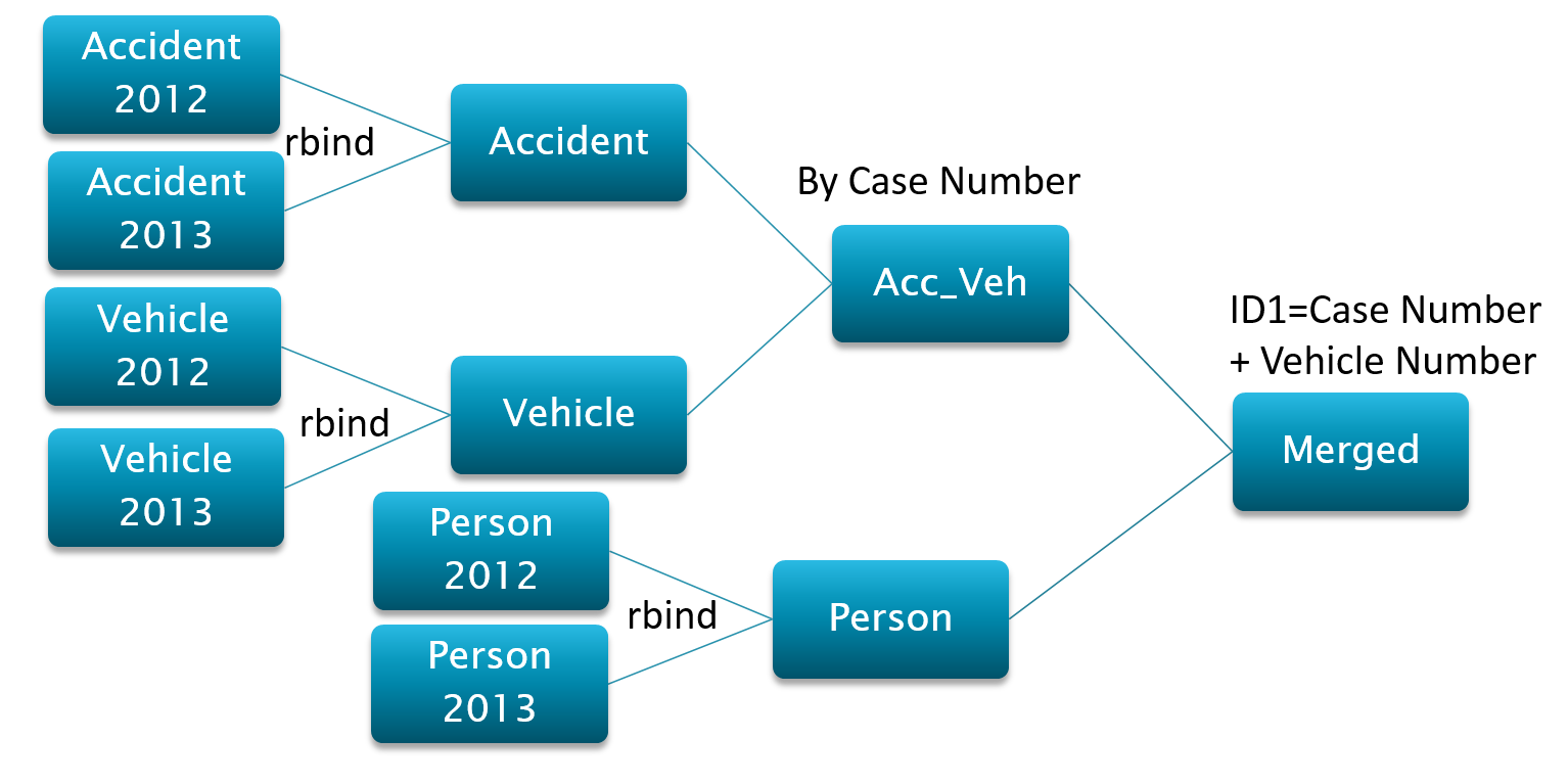
--Car safety rating
We think that certain features and conditions of the vehicle might have an influence in the maximum injury level that could have occurred in an accident. Thus, we decide to add a car safety ratings column corresponding to the specific vehicle involved in the accident. We tried to pull data through the website of U.S. Department Transportation. We found the data from 1990 to 2014. But the data is raw so we need to do something to make it useful. There are so many different types of cars and thus a lot of needless information. For simplifying, we decided to focus on Year, Make and Model of a vehicle only. Therefore, we combined the rows that have the same year, make and model. Namely, the rest information of a car, such as drive type (AWD or FWD) will not be considered any more. After importing data, we use R to do the work.
--Car crash cost by state
In order to have an accurate estimate of the economic cost of a vehicle accident, several external datasets have been brought into our original GES dataset. From the State-Specific Cost of Crash Deaths Fact Sheets, we got the total cost of crash-related deaths in each state in the year of 2013. The second external data is called Fatal Crash Totals State by State, which we got the total number of fatal crashes in each state. After dividing the cost of fatal crash in each state by the total number of fatal crash, we created a new variable called cost per crash in 2013. We then took an average of cost per crash from all the states, and we use the average number as 1 in the new column called cost adjuster. The variable of cost adjust is the index that we used to estimate the cost of the rest of the crash types. What is more, we used a national average of the average cost of Type A crash, Type B crash, Type C crash and property damage only crash. With the national average cost and the cost index, we then got the estimated cost of each type of crash in each state.
IV. Statistical Analysis
--Reasons:
The response variable is categorical with ordinal levels.
Easy to interpret for each level (Compare to Decision Tree, Neural Network).
Given survey data, we need to consider sample weights and sampling units.
--Explanatory Variables:
--Response Variable: Maximum injury severity (Binned)

--Parameter Estimates:
| Analysis of Maximum Likelihood Estimates | |||||||
|---|---|---|---|---|---|---|---|
| Parameter | SEV | DF | Estimate | Standard Error |
Wald Chi-Square |
Pr > ChiSq | |
| Intercept | Fatal | 1 | -7.4259 | 0.6789 | 119.6389 | <.0001 | |
| Intercept | TypeA | 1 | -4.0718 | 0.3332 | 149.2945 | <.0001 | |
| Intercept | TypeB | 1 | -2.8512 | 0.2386 | 142.7981 | <.0001 | |
| Intercept | TypeC | 1 | -1.9481 | 0.1777 | 120.2266 | <.0001 | |
| IMP_TRAV_SP | Fatal | 1 | 0.0437 | 0.00301 | 210.7428 | <.0001 | |
| IMP_TRAV_SP | TypeA | 1 | 0.0250 | 0.00153 | 267.2686 | <.0001 | |
| IMP_TRAV_SP | TypeB | 1 | 0.0178 | 0.00164 | 116.7216 | <.0001 | |
| IMP_TRAV_SP | TypeC | 1 | 0.00391 | 0.00150 | 6.8083 | 0.0091 | |
| IMP_VE_TOTAL | Fatal | 1 | 0.5447 | 0.1533 | 12.6253 | 0.0004 | |
| IMP_VE_TOTAL | TypeA | 1 | 0.3339 | 0.0569 | 34.4964 | <.0001 | |
| IMP_VE_TOTAL | TypeB | 1 | 0.4735 | 0.0289 | 268.8647 | <.0001 | |
| IMP_VE_TOTAL | TypeC | 1 | 0.4740 | 0.0313 | 229.9680 | <.0001 | |
| IMP_HOUR_IM | Fatal | 1 | -0.00891 | 0.00950 | 0.8813 | 0.3478 | |
| IMP_HOUR_IM | TypeA | 1 | -0.00696 | 0.00409 | 2.8951 | 0.0889 | |
| IMP_HOUR_IM | TypeB | 1 | -0.00122 | 0.00273 | 0.2006 | 0.6542 | |
| IMP_HOUR_IM | TypeC | 1 | 0.00186 | 0.00329 | 0.3191 | 0.5721 | |
| IMP_VSPD_LIM | Fatal | 1 | -0.00523 | 0.0117 | 0.1990 | 0.6555 | |
| IMP_VSPD_LIM | TypeA | 1 | -0.00506 | 0.00298 | 2.8924 | 0.0890 | |
| IMP_VSPD_LIM | TypeB | 1 | -0.00915 | 0.00264 | 12.0560 | 0.0005 | |
| IMP_VSPD_LIM | TypeC | 1 | 0.000573 | 0.00276 | 0.0429 | 0.8359 | |
| IMP_SEX_IM | 2 | Fatal | 1 | -0.2408 | 0.0642 | 14.0835 | 0.0002 |
| IMP_SEX_IM | 2 | TypeA | 1 | -0.0249 | 0.0292 | 0.7296 | 0.3930 |
| IMP_SEX_IM | 2 | TypeB | 1 | 0.0959 | 0.0173 | 30.7440 | <.0001 |
| IMP_SEX_IM | 2 | TypeC | 1 | 0.1885 | 0.0186 | 102.2626 | <.0001 |
| IMP_VSURCOND | 0 | Fatal | 1 | 0.2439 | 0.4527 | 0.2902 | 0.5901 |
| IMP_VSURCOND | 0 | TypeA | 1 | -0.0921 | 0.1729 | 0.2837 | 0.5943 |
| IMP_VSURCOND | 0 | TypeB | 1 | -0.0945 | 0.0979 | 0.9312 | 0.3346 |
| IMP_VSURCOND | 0 | TypeC | 1 | -0.2000 | 0.0985 | 4.1191 | 0.0424 |
| IMP_VSURCOND | 2 | Fatal | 1 | -0.2961 | 0.1313 | 5.0893 | 0.0241 |
| IMP_VSURCOND | 2 | TypeA | 1 | -0.2221 | 0.0766 | 8.4014 | 0.0037 |
| IMP_VSURCOND | 2 | TypeB | 1 | -0.0709 | 0.0404 | 3.0721 | 0.0796 |
| IMP_VSURCOND | 2 | TypeC | 1 | 0.00447 | 0.0417 | 0.0115 | 0.9145 |
| IMP_VSURCOND | 3 | Fatal | 1 | -0.7170 | 0.4807 | 2.2251 | 0.1358 |
| IMP_VSURCOND | 3 | TypeA | 1 | -0.7073 | 0.1533 | 21.2966 | <.0001 |
| IMP_VSURCOND | 3 | TypeB | 1 | -0.5476 | 0.1804 | 9.2095 | 0.0024 |
| IMP_VSURCOND | 3 | TypeC | 1 | -0.1994 | 0.1094 | 3.3245 | 0.0683 |
| IMP_VSURCOND | 4 | Fatal | 1 | -0.2940 | 0.5883 | 0.2498 | 0.6172 |
| IMP_VSURCOND | 4 | TypeA | 1 | -0.1082 | 0.2507 | 0.1864 | 0.6659 |
| IMP_VSURCOND | 4 | TypeB | 1 | -0.1770 | 0.1842 | 0.9235 | 0.3365 |
| IMP_VSURCOND | 4 | TypeC | 1 | -0.0963 | 0.1303 | 0.5460 | 0.4600 |
| IMP_VSURCOND | 5 | Fatal | 1 | 1.9986 | 0.9485 | 4.4399 | 0.0351 |
| IMP_VSURCOND | 5 | TypeA | 1 | -0.1512 | 1.0079 | 0.0225 | 0.8807 |
| IMP_VSURCOND | 5 | TypeB | 1 | 1.7020 | 0.4147 | 16.8418 | <.0001 |
| IMP_VSURCOND | 5 | TypeC | 1 | -0.5725 | 0.6821 | 0.7045 | 0.4013 |
| IMP_VSURCOND | 6 | Fatal | 1 | -7.6101 | 0.2264 | 1130.1624 | <.0001 |
| IMP_VSURCOND | 6 | TypeA | 1 | -0.4166 | 0.4835 | 0.7424 | 0.3889 |
| IMP_VSURCOND | 6 | TypeB | 1 | -0.1424 | 0.2561 | 0.3090 | 0.5783 |
| IMP_VSURCOND | 6 | TypeC | 1 | 0.3034 | 0.2900 | 1.0945 | 0.2955 |
| IMP_VSURCOND | 7 | Fatal | 1 | -9.8958 | 0.6651 | 221.3908 | <.0001 |
| IMP_VSURCOND | 7 | TypeA | 1 | 3.0866 | 0.9464 | 10.6373 | 0.0011 |
| IMP_VSURCOND | 7 | TypeB | 1 | 2.7599 | 0.7791 | 12.5478 | 0.0004 |
| IMP_VSURCOND | 7 | TypeC | 1 | 2.1229 | 0.8017 | 7.0122 | 0.0081 |
| IMP_VSURCOND | 8 | Fatal | 1 | 0.5991 | 0.9389 | 0.4072 | 0.5234 |
| IMP_VSURCOND | 8 | TypeA | 1 | -0.2379 | 0.4093 | 0.3378 | 0.5611 |
| IMP_VSURCOND | 8 | TypeB | 1 | -1.0340 | 0.4175 | 6.1326 | 0.0133 |
| IMP_VSURCOND | 8 | TypeC | 1 | 0.1314 | 0.6673 | 0.0387 | 0.8440 |
| IMP_VSURCOND | 10 | Fatal | 1 | 0.2950 | 0.9060 | 0.1060 | 0.7448 |
| IMP_VSURCOND | 10 | TypeA | 1 | 0.5769 | 0.5274 | 1.1964 | 0.2740 |
| IMP_VSURCOND | 10 | TypeB | 1 | -0.1235 | 0.4046 | 0.0932 | 0.7602 |
| IMP_VSURCOND | 10 | TypeC | 1 | -0.3136 | 0.1813 | 2.9910 | 0.0837 |
| IMP_VSURCOND | 11 | Fatal | 1 | 0.9102 | 0.5553 | 2.6863 | 0.1012 |
| IMP_VSURCOND | 11 | TypeA | 1 | 0.9708 | 0.5045 | 3.7026 | 0.0543 |
| IMP_VSURCOND | 11 | TypeB | 1 | 0.3795 | 0.2049 | 3.4293 | 0.0641 |
| IMP_VSURCOND | 11 | TypeC | 1 | -0.3508 | 0.4601 | 0.5814 | 0.4457 |
| IMP_VSURCOND | 9999 | Fatal | 1 | -0.3257 | 0.5982 | 0.2964 | 0.5862 |
| IMP_VSURCOND | 9999 | TypeA | 1 | -1.4482 | 0.3909 | 13.7292 | 0.0002 |
| IMP_VSURCOND | 9999 | TypeB | 1 | -1.2454 | 0.2747 | 20.5476 | <.0001 |
| IMP_VSURCOND | 9999 | TypeC | 1 | -0.9124 | 0.1973 | 21.3917 | <.0001 |
| REGION | 2 | Fatal | 1 | 0.2511 | 0.3193 | 0.6183 | 0.4317 |
| REGION | 2 | TypeA | 1 | 0.1046 | 0.1476 | 0.5024 | 0.4785 |
| REGION | 2 | TypeB | 1 | 0.3519 | 0.1923 | 3.3491 | 0.0672 |
| REGION | 2 | TypeC | 1 | -0.4874 | 0.1403 | 12.0703 | 0.0005 |
| REGION | 3 | Fatal | 1 | 0.2416 | 0.2975 | 0.6597 | 0.4167 |
| REGION | 3 | TypeA | 1 | 0.2395 | 0.2151 | 1.2391 | 0.2656 |
| REGION | 3 | TypeB | 1 | 0.3612 | 0.2137 | 2.8575 | 0.0909 |
| REGION | 3 | TypeC | 1 | -0.3170 | 0.1702 | 3.4708 | 0.0625 |
| REGION | 4 | Fatal | 1 | 0.7223 | 0.3218 | 5.0374 | 0.0248 |
| REGION | 4 | TypeA | 1 | 0.3549 | 0.1984 | 3.2008 | 0.0736 |
| REGION | 4 | TypeB | 1 | 0.5830 | 0.2089 | 7.7917 | 0.0052 |
| REGION | 4 | TypeC | 1 | -0.0211 | 0.1456 | 0.0210 | 0.8849 |
| IMP_SAFETY_RATING | Fatal | 1 | -0.1740 | 0.1058 | 2.7020 | 0.1002 | |
| IMP_SAFETY_RATING | TypeA | 1 | -0.2152 | 0.0320 | 45.1180 | <.0001 | |
| IMP_SAFETY_RATING | TypeB | 1 | -0.1682 | 0.0270 | 38.7430 | <.0001 | |
| IMP_SAFETY_RATING | TypeC | 1 | -0.1235 | 0.0283 | 19.0761 | <.0001 | |
| IMP_LAND_USE | 2 | Fatal | 1 | -0.4506 | 0.3823 | 1.3896 | 0.2385 |
| IMP_LAND_USE | 2 | TypeA | 1 | -0.1101 | 0.1645 | 0.4476 | 0.5035 |
| IMP_LAND_USE | 2 | TypeB | 1 | -0.00905 | 0.1014 | 0.0080 | 0.9289 |
| IMP_LAND_USE | 2 | TypeC | 1 | -0.1108 | 0.1295 | 0.7319 | 0.3923 |
| IMP_LAND_USE | 3 | Fatal | 1 | -0.3227 | 0.2114 | 2.3298 | 0.1269 |
| IMP_LAND_USE | 3 | TypeA | 1 | 0.0502 | 0.1534 | 0.1069 | 0.7437 |
| IMP_LAND_USE | 3 | TypeB | 1 | -0.0747 | 0.1021 | 0.5351 | 0.4645 |
| IMP_LAND_USE | 3 | TypeC | 1 | 0.1651 | 0.0758 | 4.7445 | 0.0294 |
| IMP_LAND_USE | 8 | Fatal | 1 | 0.2121 | 0.1803 | 1.3838 | 0.2395 |
| IMP_LAND_USE | 8 | TypeA | 1 | 0.2737 | 0.0810 | 11.4283 | 0.0007 |
| IMP_LAND_USE | 8 | TypeB | 1 | 0.2910 | 0.0938 | 9.6167 | 0.0019 |
| IMP_LAND_USE | 8 | TypeC | 1 | 0.0988 | 0.0710 | 1.9399 | 0.1637 |
| IMP_driver_age | Fatal | 1 | 0.0118 | 0.00278 | 18.0843 | <.0001 | |
| IMP_driver_age | TypeA | 1 | 0.00556 | 0.00148 | 14.1946 | 0.0002 | |
| IMP_driver_age | TypeB | 1 | 0.00104 | 0.00128 | 0.6607 | 0.4163 | |
| IMP_driver_age | TypeC | 1 | 0.00204 | 0.000815 | 6.2645 | 0.0123 | |
| overspeed | 1 | Fatal | 1 | 0.6434 | 0.1508 | 18.2100 | <.0001 |
| overspeed | 1 | TypeA | 1 | 0.6316 | 0.1057 | 35.7132 | <.0001 |
| overspeed | 1 | TypeB | 1 | 0.5588 | 0.0801 | 48.6655 | <.0001 |
| overspeed | 1 | TypeC | 1 | 0.3216 | 0.0775 | 17.2043 | <.0001 |
| IMP_ALCHL_IM | 1 | Fatal | 1 | 2.3002 | 0.1526 | 227.2388 | <.0001 |
| IMP_ALCHL_IM | 1 | TypeA | 1 | 1.6115 | 0.0857 | 353.6302 | <.0001 |
| IMP_ALCHL_IM | 1 | TypeB | 1 | 1.0581 | 0.0795 | 177.1651 | <.0001 |
| IMP_ALCHL_IM | 1 | TypeC | 1 | 0.3848 | 0.0998 | 14.8645 | 0.0001 |
V. Results
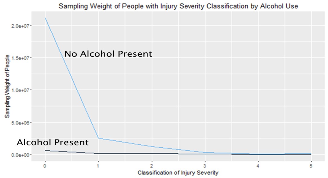
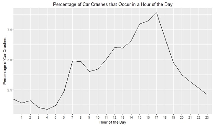
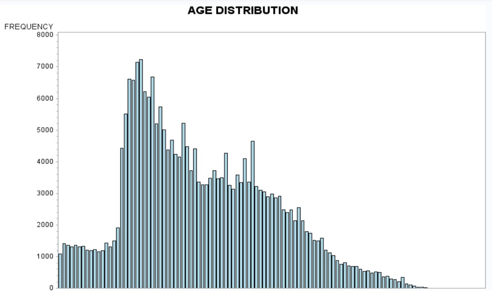
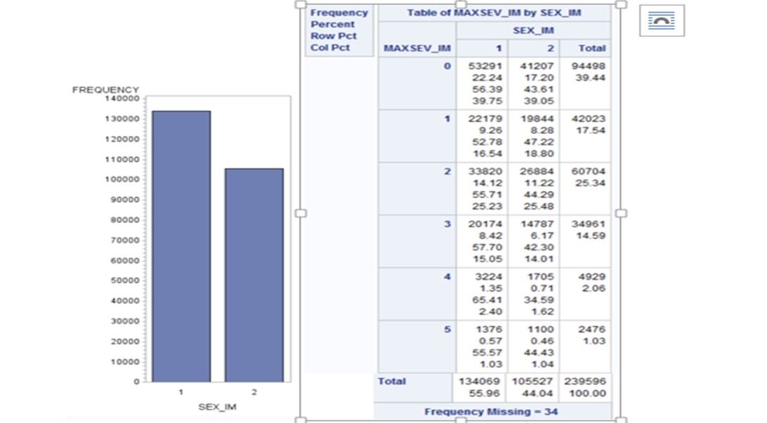
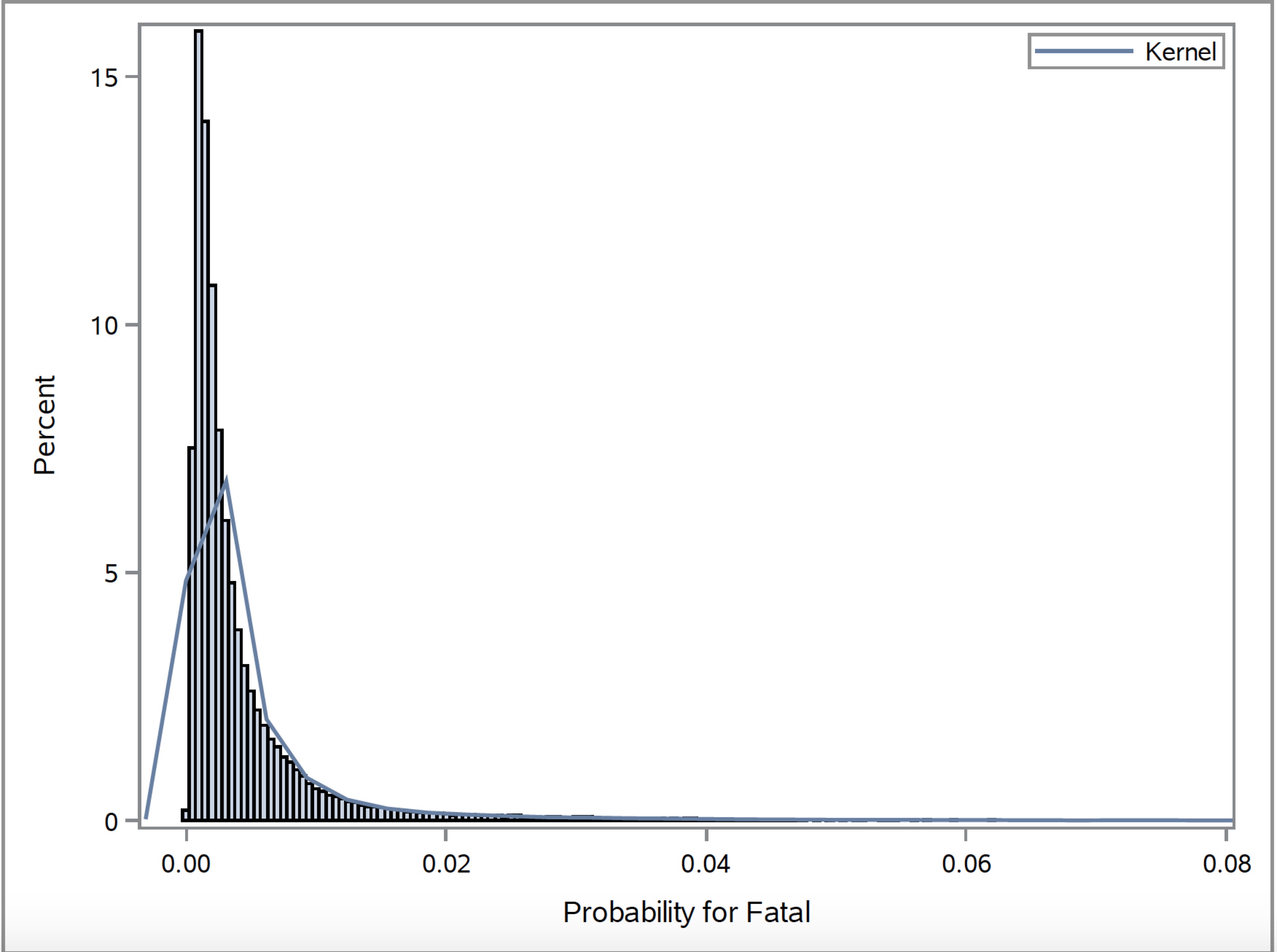
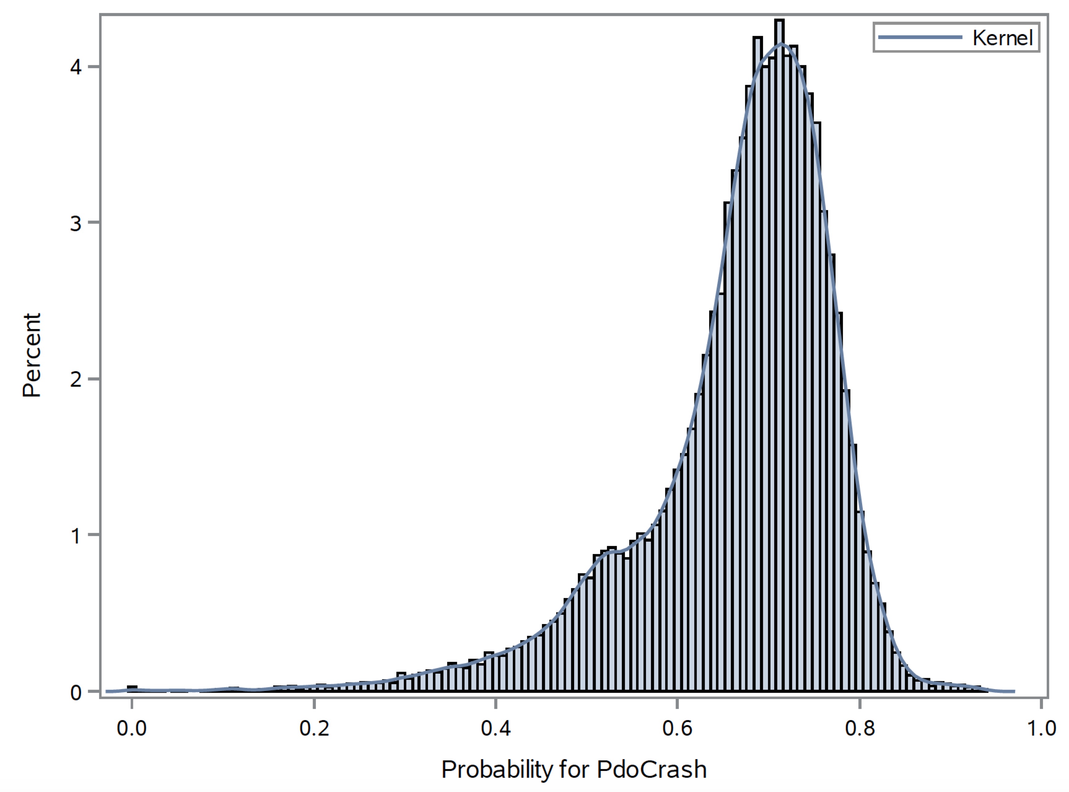
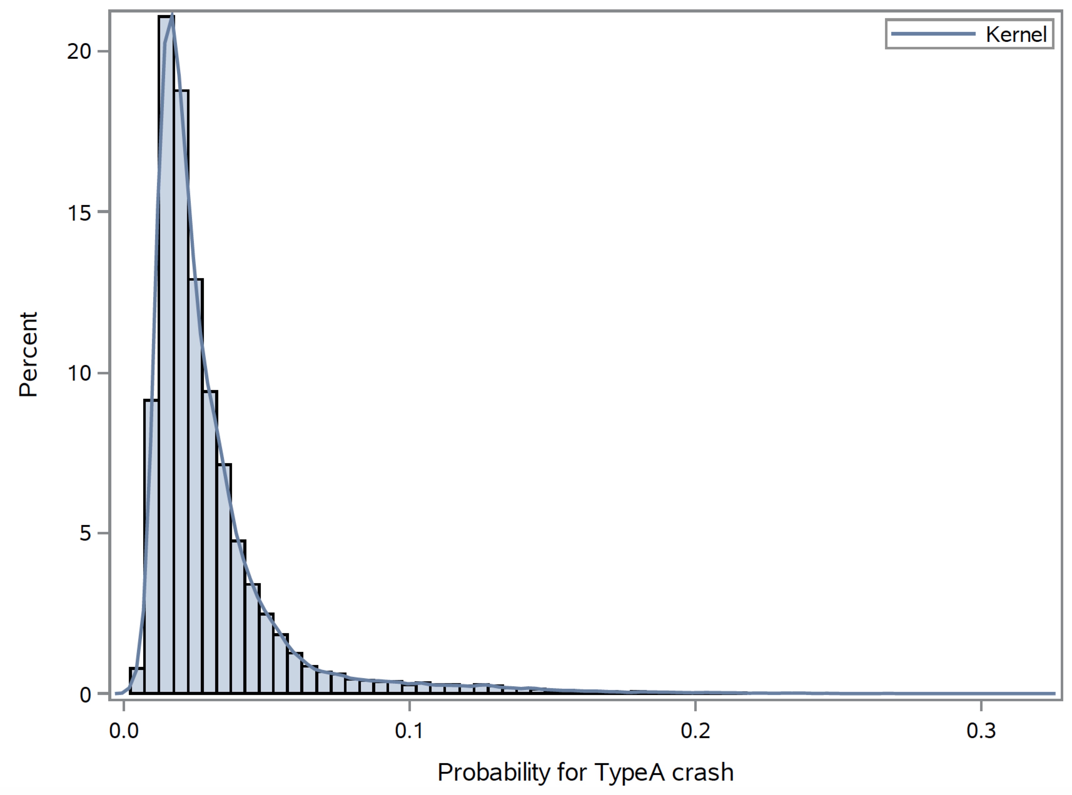
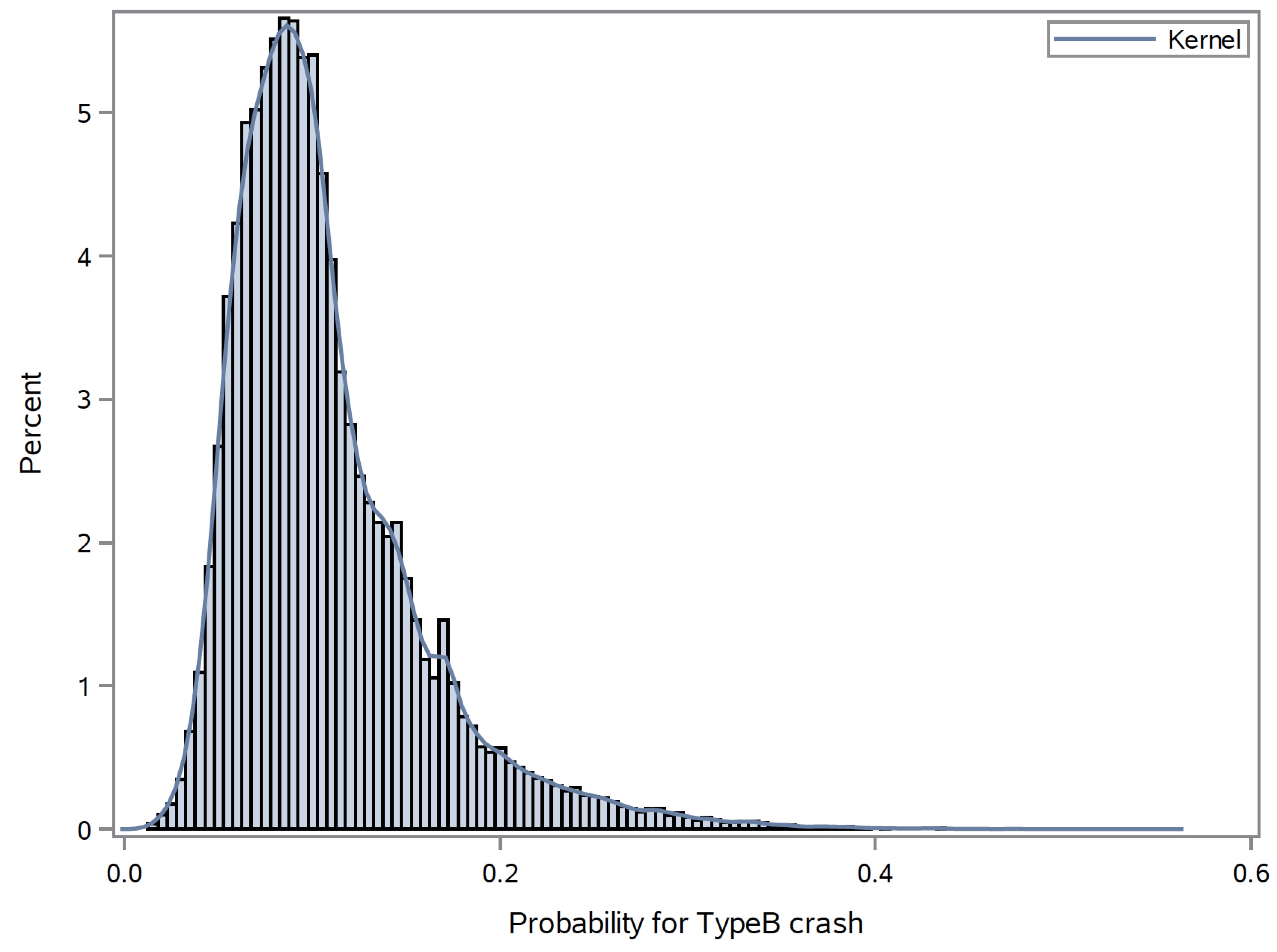
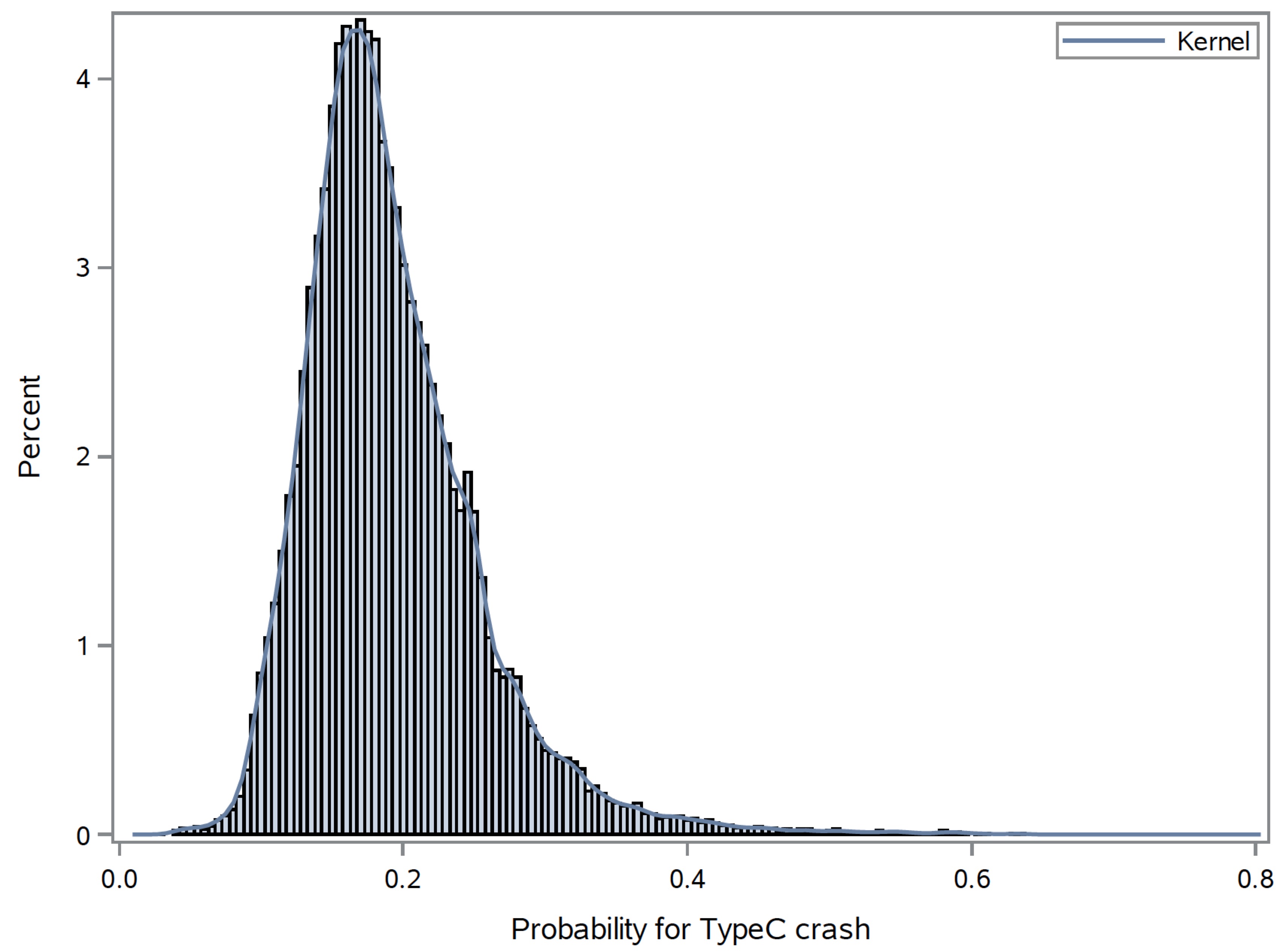
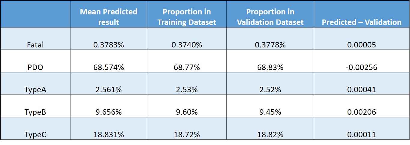
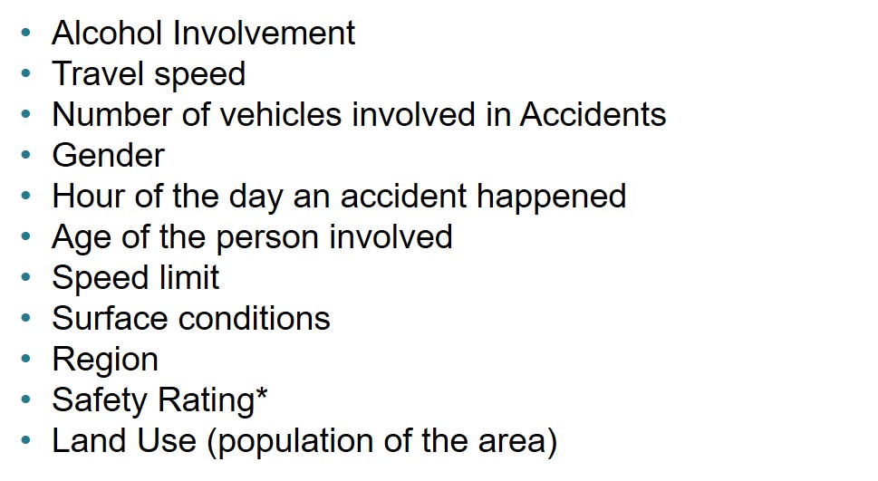
The final model includes the following variables: If alcohol was involved or not, travel speed, number of vehicles included, hour of the day, age of the person involved, speed limit, gender, surface conditions, region, safety rating of the car, and land use. By using these variables we are able to predict the maximum injury severity of individuals involved in a car accident. Once the probability of the different maximum injury severity levels has been determined, we use this to proceed. We also use the Region information combined with the outside data source to determine the economic cost of a car accident. The economic cost of a car accident takes into account the cost to the individual for medical expenses, and the cost of fixing the vehicle(s) involved in the accident. This model will not only help people better understand the costs of an accident, both physically and financially, but will hopefully assist people in making more informed decisions about the vehicles they drive and the driving behavior they exhibit on the road.
